- Главная
- Разное
- Бизнес и предпринимательство
- Образование
- Развлечения
- Государство
- Спорт
- Графика
- Культурология
- Еда и кулинария
- Лингвистика
- Религиоведение
- Черчение
- Физкультура
- ИЗО
- Психология
- Социология
- Английский язык
- Астрономия
- Алгебра
- Биология
- География
- Геометрия
- Детские презентации
- Информатика
- История
- Литература
- Маркетинг
- Математика
- Медицина
- Менеджмент
- Музыка
- МХК
- Немецкий язык
- ОБЖ
- Обществознание
- Окружающий мир
- Педагогика
- Русский язык
- Технология
- Физика
- Философия
- Химия
- Шаблоны, картинки для презентаций
- Экология
- Экономика
- Юриспруденция
Что такое findslide.org?
FindSlide.org - это сайт презентаций, докладов, шаблонов в формате PowerPoint.
Обратная связь
Email: Нажмите что бы посмотреть
Презентация на тему Image Stitching
Содержание
- 2. Combine two or more overlapping images to make one larger imageAdd exampleSlide credit: Vaibhav Vaish
- 3. How to do it?Basic ProcedureTake a sequence
- 4. 1. Take a sequence of images from
- 5. 2. Compute transformation between imagesExtract interest pointsFind MatchesCompute transformation?
- 6. 3. Shift the images to overlap
- 7. 4. Blend the two together to create a mosaic
- 8. 5. Repeat for all images
- 9. How to do it?Basic ProcedureTake a sequence
- 10. Compute TransformationsExtract interest pointsFind good matches Compute
- 11. Image reprojectionThe mosaic has a natural interpretation
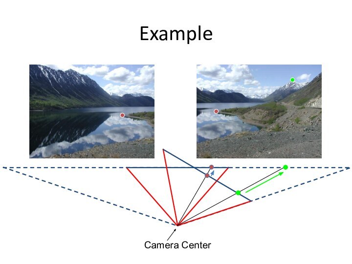
- 12. ExampleCamera Center
- 13. Image reprojectionObservationRather than thinking of this as
- 14. Motion modelsWhat happens when we take two images with a camera and try to align them?translation?rotation?scale?affine?Perspective?
- 15. Recall: Projective transformations(aka homographies)
- 16. Parametric (global) warpingExamples of parametric warps:translationrotationaspectaffineperspective
- 17. 2D coordinate transformationstranslation: x’ = x + t
- 18. Image WarpingGiven a coordinate transform x’ =
- 19. Forward WarpingSend each pixel f(x) to its
- 20. Forward WarpingSend each pixel f(x) to its
- 21. Richard SzeliskiImage StitchingInverse WarpingGet each pixel g(x’)
- 22. Richard SzeliskiImage StitchingInverse WarpingGet each pixel g(x’)
- 23. InterpolationPossible interpolation filters:nearest neighborbilinearbicubic (interpolating)
- 24. Motion models
- 25. Finding the transformationTranslation = 2 degrees of
- 26. Plane perspective mosaics8-parameter generalization of affine motionworks
- 27. Simple case: translations
- 28. Simple case: translations
- 29. Simple case: translationsSystem of linear equationsWhat are
- 30. Simple case: translationsProblem: more equations than unknowns“Overdetermined” system of equationsWe will find the least squares solution
- 31. Least squares formulationFor each pointwe define the residuals as
- 32. Least squares formulationGoal: minimize sum of squared residuals“Least squares” solutionFor translations, is equal to mean displacement
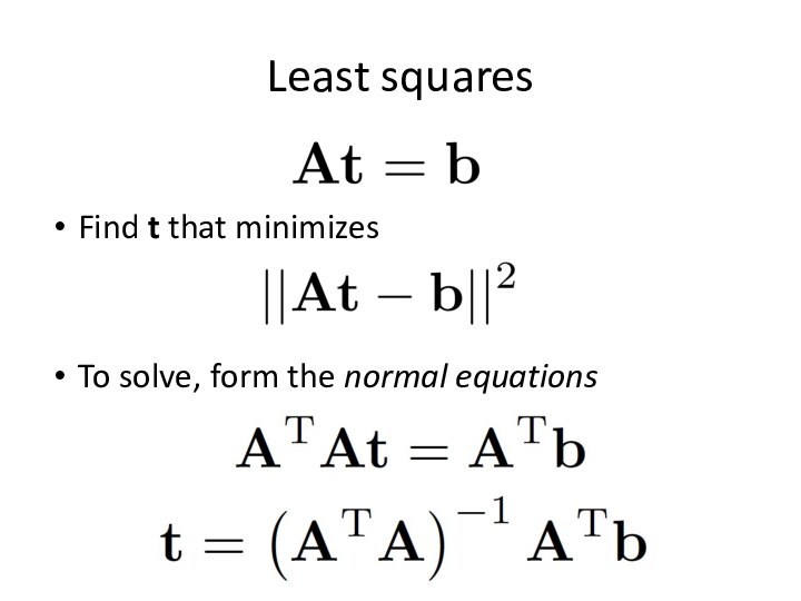
- 33. Least squaresFind t that minimizes To solve, form the normal equations
- 34. Solving for translationsUsing least squares
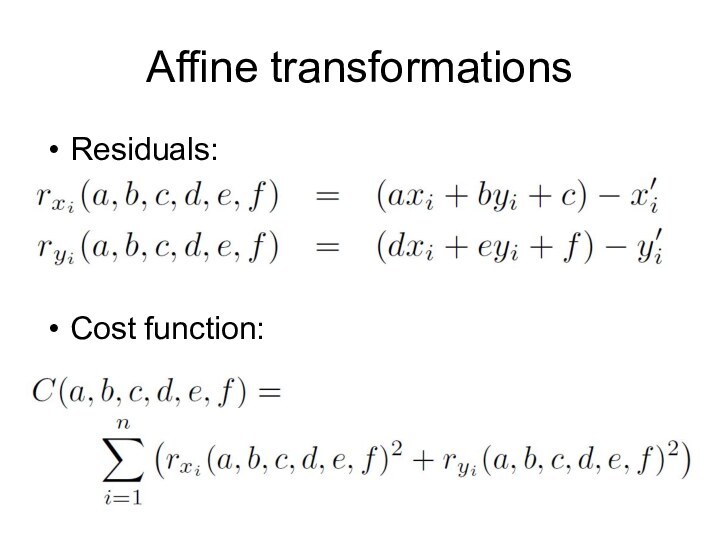
- 35. Affine transformationsHow many unknowns?How many equations per match?How many matches do we need?
- 36. Affine transformationsResiduals:Cost function:
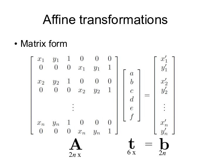
- 37. Affine transformationsMatrix form
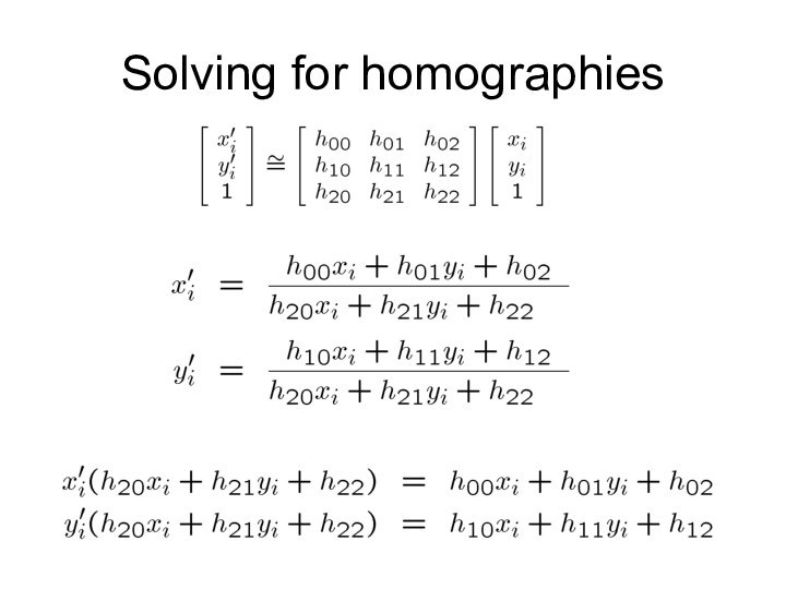
- 38. Solving for homographies
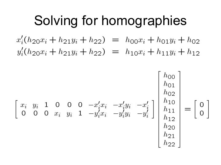
- 39. Solving for homographies
- 40. Direct Linear TransformsDefines a least squares problem:Since
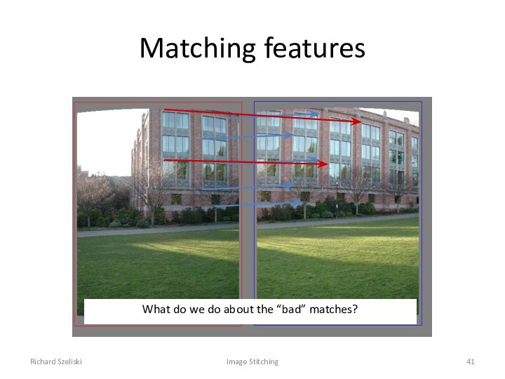
- 41. Richard SzeliskiImage StitchingMatching featuresWhat do we do about the “bad” matches?
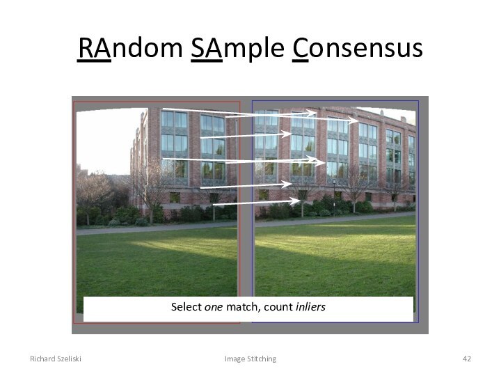
- 42. Richard SzeliskiImage StitchingRAndom SAmple ConsensusSelect one match, count inliers
- 43. Richard SzeliskiImage StitchingRAndom SAmple ConsensusSelect one match, count inliers
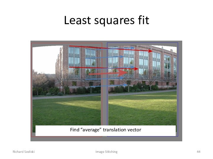
- 44. Richard SzeliskiImage StitchingLeast squares fitFind “average” translation vector
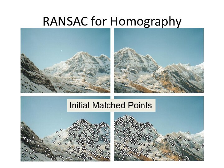
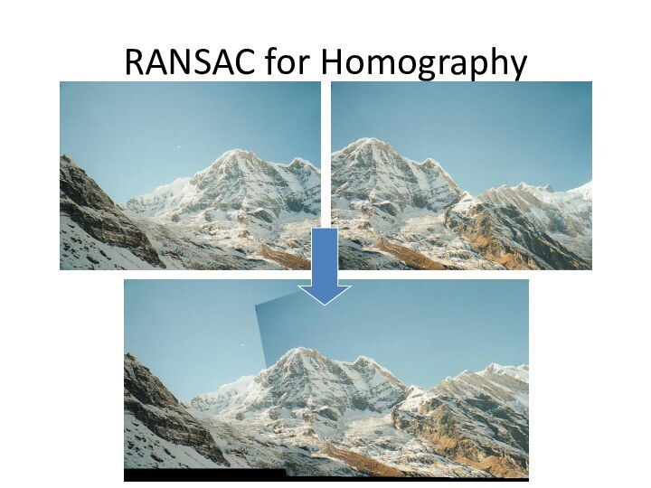
- 46. RANSAC for estimating homographyRANSAC loop:Select four feature
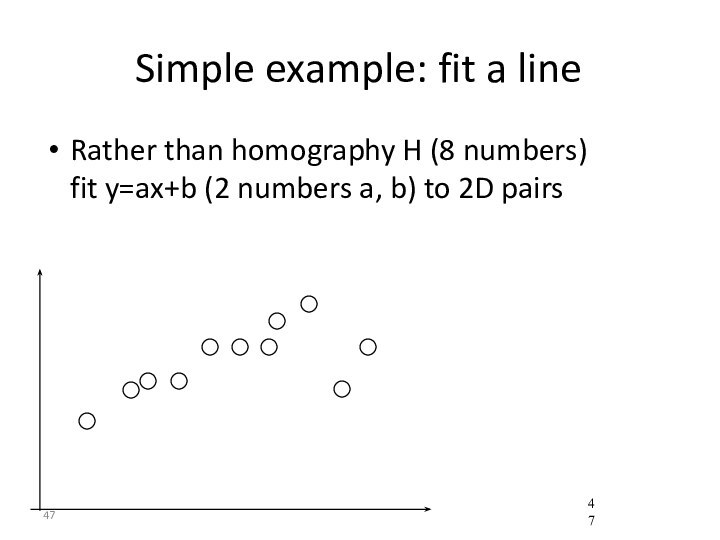
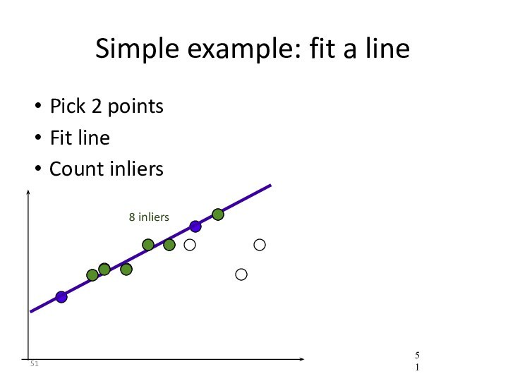
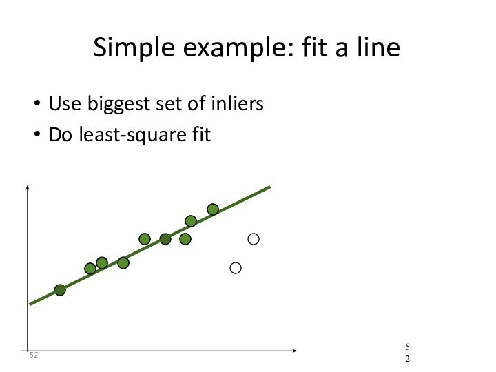
- 47. Simple example: fit a lineRather than homography
- 48. Simple example: fit a linePick 2 pointsFit lineCount inliers3 inliers
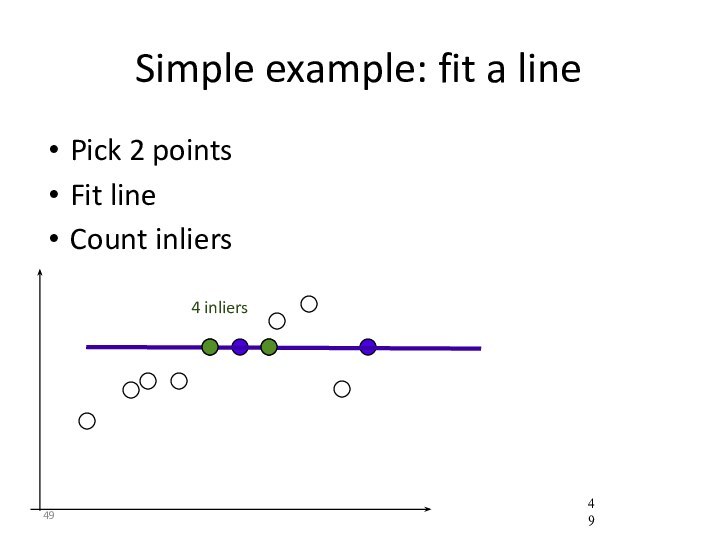
- 49. Simple example: fit a linePick 2 pointsFit lineCount inliers4 inliers
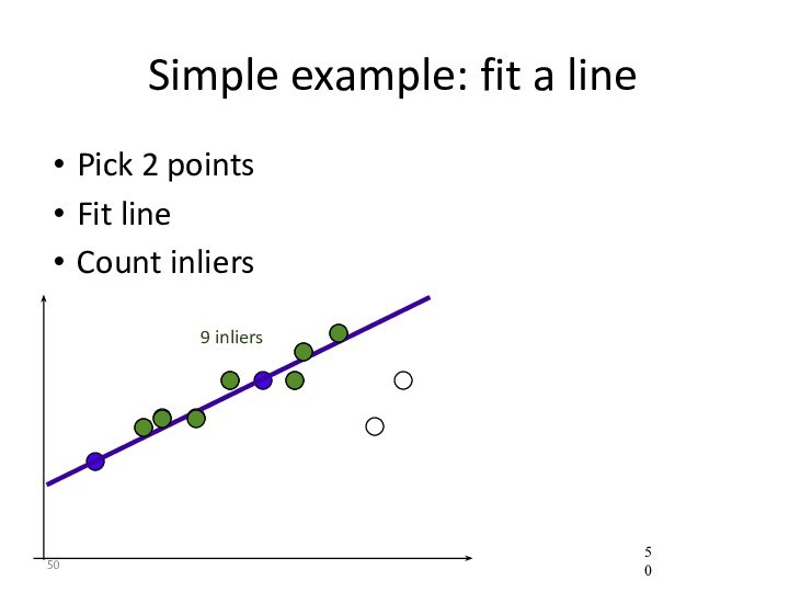
- 50. Simple example: fit a linePick 2 pointsFit lineCount inliers9 inliers
- 51. Simple example: fit a linePick 2 pointsFit lineCount inliers8 inliers
- 52. Simple example: fit a lineUse biggest set of inliersDo least-square fit
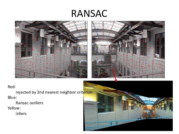
- 53. RANSACRed: rejected by 2nd nearest neighbor criterionBlue: Ransac outliersYellow: inliers
- 54. How many rounds? If we have to
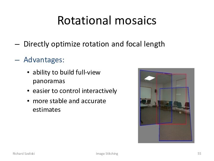
- 55. Richard SzeliskiImage StitchingRotational mosaicsDirectly optimize rotation and
- 56. Richard SzeliskiImage StitchingRotational mosaicProjection equationsProject from image
- 57. Computing homographyAssume we have four matched points:
- 58. Computing homographyAssume we have matched points with
- 59. Automatic Image StitchingCompute interest points on each
- 60. RANSAC for HomographyInitial Matched Points
- 61. RANSAC for HomographyFinal Matched Points
- 62. Скачать презентацию
- 63. Похожие презентации
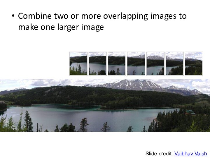
Combine two or more overlapping images to make one larger imageAdd exampleSlide credit: Vaibhav Vaish





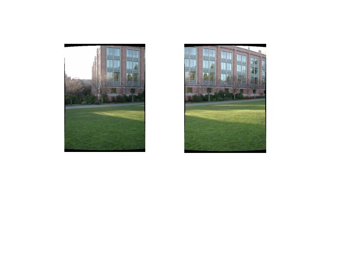




Слайд 3
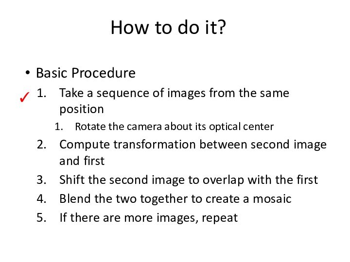
How to do it?
Basic Procedure
Take a sequence of
images from the same position
Rotate the camera about its
optical centerCompute transformation between second image and first
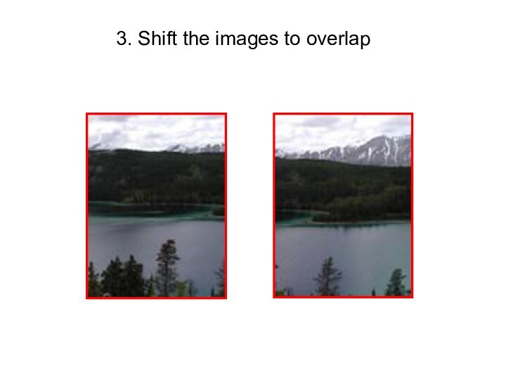
Shift the second image to overlap with the first
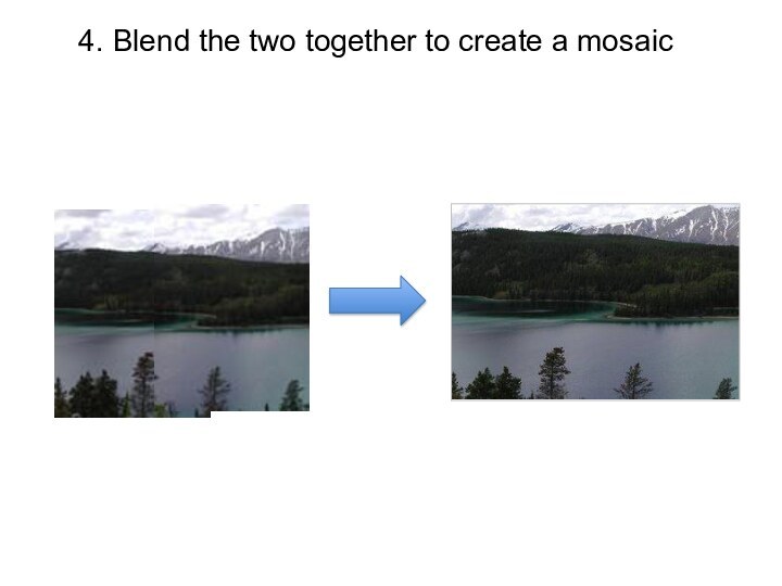
Blend the two together to create a mosaic
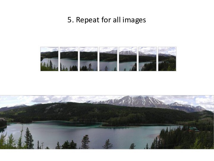
If there are more images, repeat
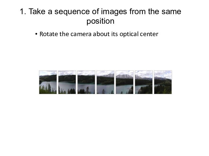
Слайд 4 1. Take a sequence of images from the
same position
Rotate the camera about its optical center
Слайд 5
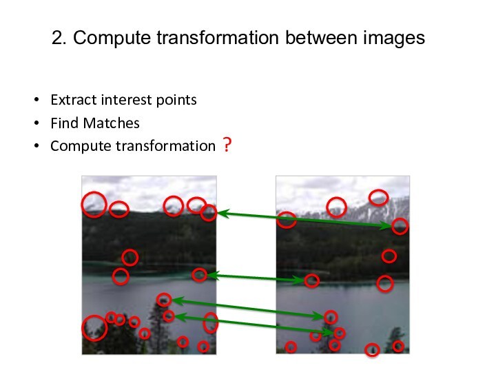
2. Compute transformation between images
Extract interest points
Find Matches
Compute
transformation
?
Слайд 9
How to do it?
Basic Procedure
Take a sequence of
images from the same position
Rotate the camera about its
optical centerCompute transformation between second image and first
Shift the second image to overlap with the first
Blend the two together to create a mosaic
If there are more images, repeat
✓
Слайд 10
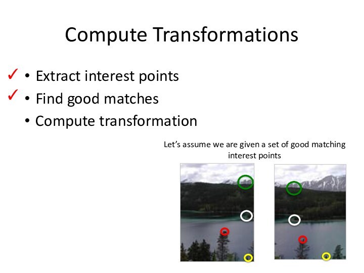
Compute Transformations
Extract interest points
Find good matches
Compute transformation
✓
Let’s
assume we are given a set of good matching
interest points✓
Слайд 11
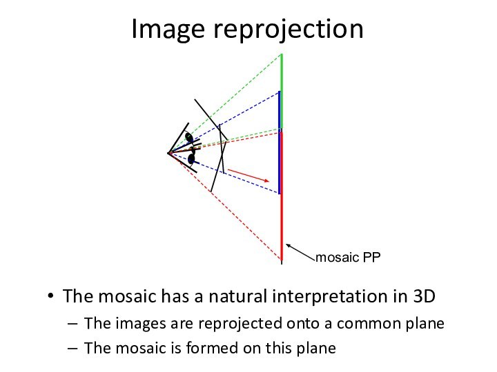
Image reprojection
The mosaic has a natural interpretation in
3D
The images are reprojected onto a common plane
The mosaic
is formed on this plane
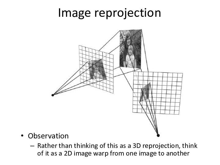
Слайд 13
Image reprojection
Observation
Rather than thinking of this as a
3D reprojection, think of it as a 2D image
warp from one image to another
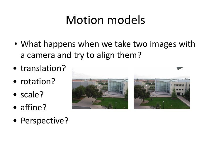
Слайд 14
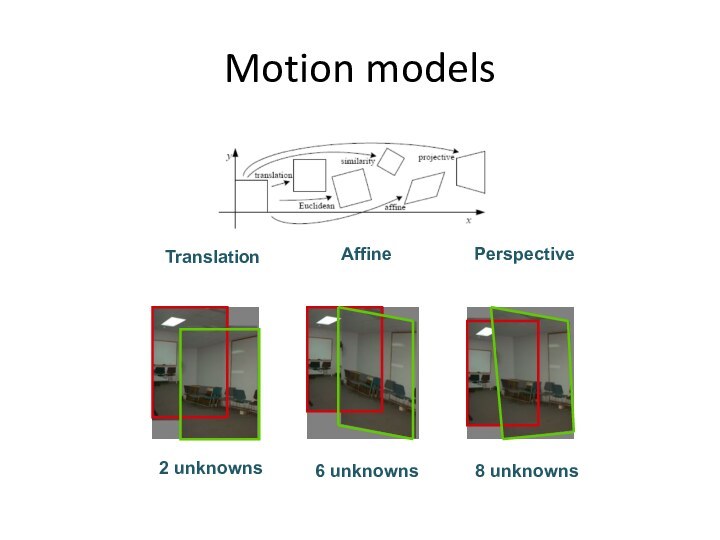
Motion models
What happens when we take two images
with a camera and try to align them?
translation?
rotation?
scale?
affine?
Perspective?
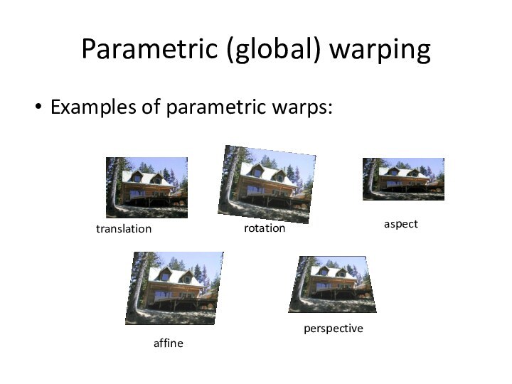
Слайд 16
Parametric (global) warping
Examples of parametric warps:
translation
rotation
aspect
affine
perspective
Слайд 17
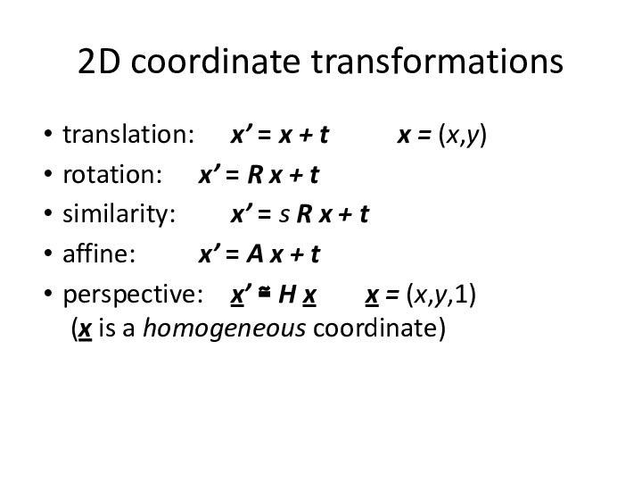
2D coordinate transformations
translation: x’ = x + t x
= (x,y)
rotation: x’ = R x + t
similarity: x’ = s
R x + taffine: x’ = A x + t
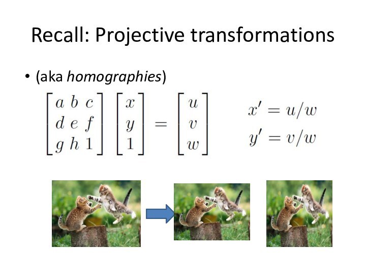
perspective: x’ ≅ H x x = (x,y,1) (x is a homogeneous coordinate)
Слайд 18
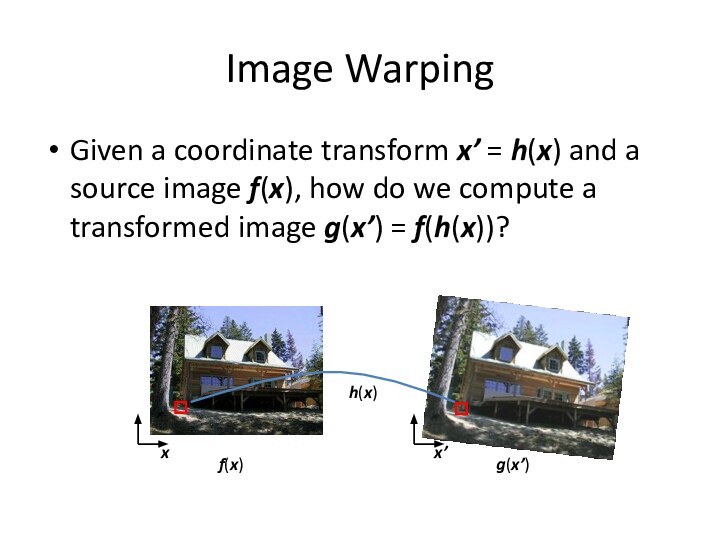
Image Warping
Given a coordinate transform x’ = h(x)
and a source image f(x), how do we compute
a transformed image g(x’) = f(h(x))?f(x)
g(x’)
x
x’
h(x)
Слайд 19
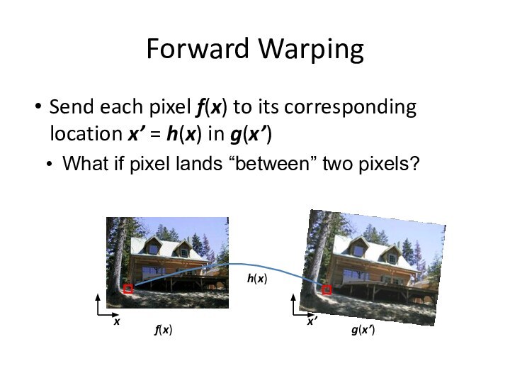
Forward Warping
Send each pixel f(x) to its corresponding
location x’ = h(x) in g(x’)
f(x)
g(x’)
x
x’
h(x)
What if pixel lands
“between” two pixels?
Слайд 20
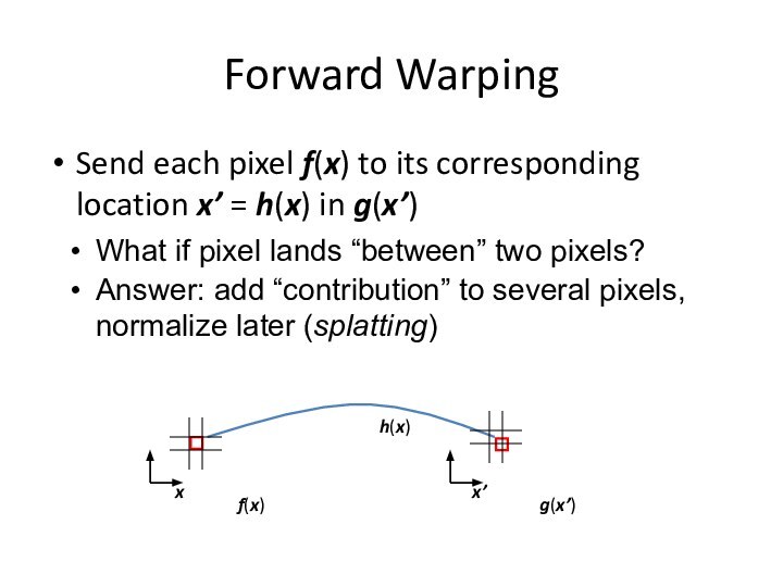
Forward Warping
Send each pixel f(x) to its corresponding
location x’ = h(x) in g(x’)
f(x)
g(x’)
x
x’
h(x)
What if pixel lands
“between” two pixels?Answer: add “contribution” to several pixels, normalize later (splatting)
Слайд 21
Richard Szeliski
Image Stitching
Inverse Warping
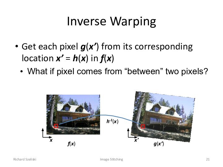
Get each pixel g(x’) from
its corresponding location x’ = h(x) in f(x)
f(x)
g(x’)
x
x’
h-1(x)
What if
pixel comes from “between” two pixels?
Слайд 22
Richard Szeliski
Image Stitching
Inverse Warping
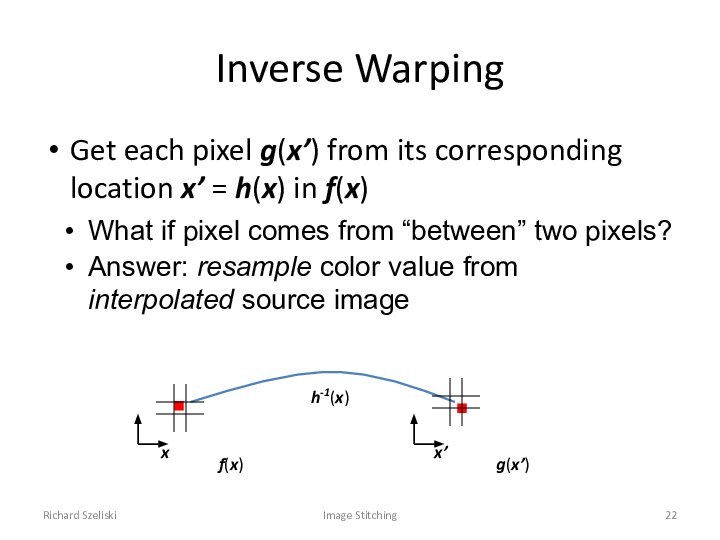
Get each pixel g(x’) from
its corresponding location x’ = h(x) in f(x)
What if
pixel comes from “between” two pixels?Answer: resample color value from interpolated source image
f(x)
g(x’)
x
x’
h-1(x)
Слайд 23
Interpolation
Possible interpolation filters:
nearest neighbor
bilinear
bicubic (interpolating)
Слайд 25
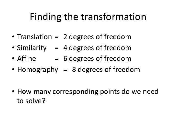
Finding the transformation
Translation = 2 degrees of freedom
Similarity
= 4 degrees of freedom
Affine = 6 degrees of
freedomHomography = 8 degrees of freedom
How many corresponding points do we need to solve?
Слайд 26
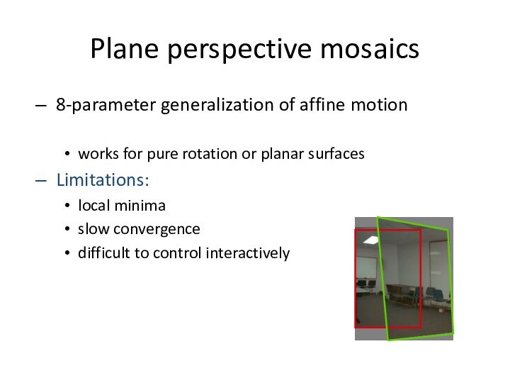
Plane perspective mosaics
8-parameter generalization of affine motion
works for
pure rotation or planar surfaces
Limitations:
local minima
slow convergence
difficult to
control interactively
Слайд 29
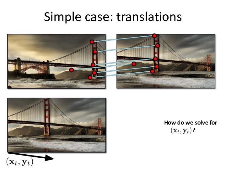
Simple case: translations
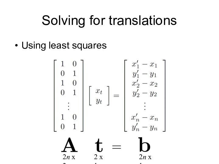
System of linear equations
What are the
knowns? Unknowns?
How many unknowns? How many equations (per match)?
Слайд 30
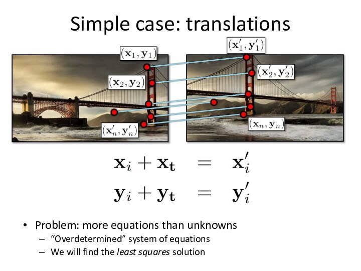
Simple case: translations
Problem: more equations than unknowns
“Overdetermined” system
of equations
We will find the least squares solution
Слайд 32
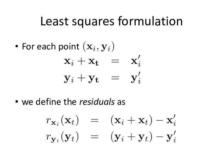
Least squares formulation
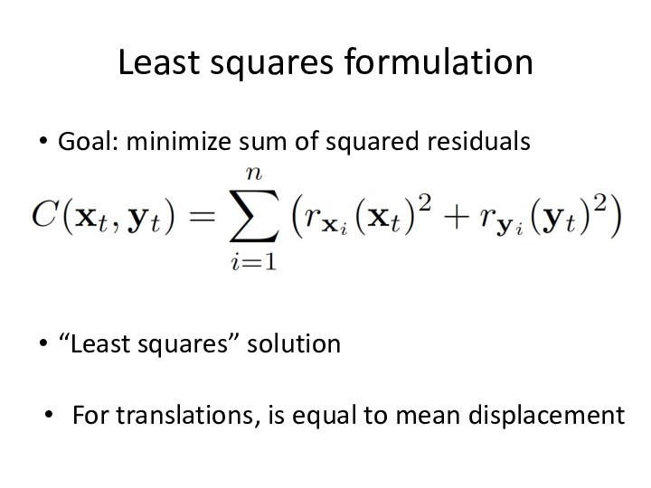
Goal: minimize sum of squared residuals
“Least
squares” solution
For translations, is equal to mean displacement
Слайд 35
Affine transformations
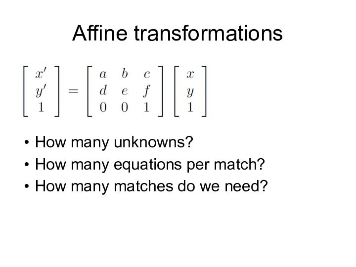
How many unknowns?
How many equations per match?
How
many matches do we need?
Слайд 40
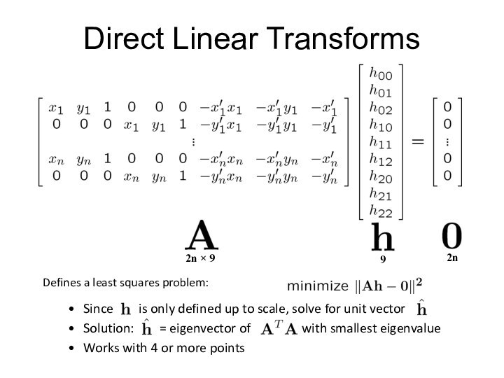
Direct Linear Transforms
Defines a least squares problem:
Since
is only defined up to scale, solve
for unit vectorSolution: = eigenvector of with smallest eigenvalue
Works with 4 or more points
Слайд 46
RANSAC for estimating homography
RANSAC loop:
Select four feature pairs
(at random)
Compute homography H (exact)
Compute inliers where ||pi’, H
pi|| < εKeep largest set of inliers
Re-compute least-squares H estimate using all of the inliers
CSE 576, Spring 2008
Structure from Motion
Слайд 47
Simple example: fit a line
Rather than homography H
(8 numbers) fit y=ax+b (2 numbers a, b) to
2D pairs
Слайд 54
How many rounds?
If we have to choose
s samples each time
with an outlier ratio e
and we
want the right answer with probability p
Слайд 55
Richard Szeliski
Image Stitching
Rotational mosaics
Directly optimize rotation and focal
length
Advantages:
ability to build full-view
panoramas
easier to control interactively
more stable
and accurate
estimates
Слайд 56
Richard Szeliski
Image Stitching
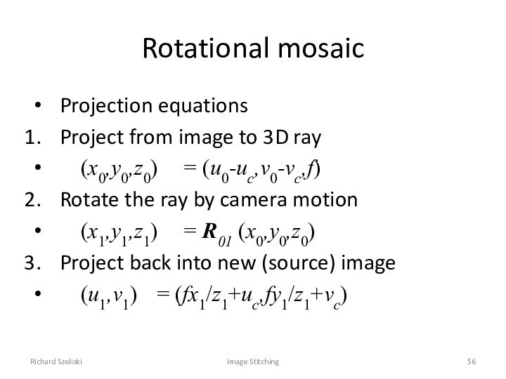
Rotational mosaic
Projection equations
Project from image to
3D ray
(x0,y0,z0) = (u0-uc,v0-vc,f)
Rotate the ray by camera motion
(x1,y1,z1)
= R01 (x0,y0,z0)Project back into new (source) image
(u1,v1) = (fx1/z1+uc,fy1/z1+vc)
Слайд 57
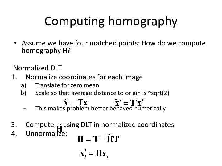
Computing homography
Assume we have four matched points: How
do we compute homography H?
Normalized DLT
Normalize coordinates for each
imageTranslate for zero mean
Scale so that average distance to origin is ~sqrt(2)
This makes problem better behaved numerically
Compute using DLT in normalized coordinates
Unnormalize:
Слайд 58
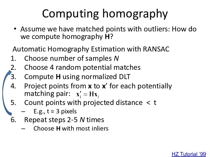
Computing homography
Assume we have matched points with outliers:
How do we compute homography H?
Automatic Homography Estimation with
RANSACChoose number of samples N
Choose 4 random potential matches
Compute H using normalized DLT
Project points from x to x’ for each potentially matching pair:
Count points with projected distance < t
E.g., t = 3 pixels
Repeat steps 2-5 N times
Choose H with most inliers
HZ Tutorial ‘99
Слайд 59
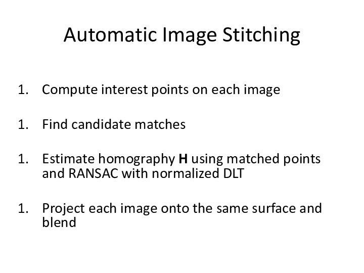
Automatic Image Stitching
Compute interest points on each image
Find
candidate matches
Estimate homography H using matched points and RANSAC
with normalized DLTProject each image onto the same surface and blend
