Слайд 2
Transient Brake Rotor
This case models the transient heating
of a steel rear disk brake rotor on a
car as it brakes from 60 to 0 mph in 3.6 seconds.
To keep solution times to a minimum the case has been simplified by removing the wheel and brake assembly to leave only the brake rotor. The brake pad is modeled by applying a heat source to a small region of the brake rotor.
Слайд 3
Assumptions
The ambient air temperature is 81 F and
the rotor is at ambient temperature before braking begins
The
vehicle tire size is 205/55/R16
The total vehicle weight including passengers and cargo is 1609 kg
The entire kinetic energy of the vehicle is dissipated through the brake rotors
Energy dissipation during braking is split 70/30 between the front and rear brakes and split evenly between the left and right sides
The vehicles speed reduces linearly from 60 to 0 mph in 3.6 seconds
Слайд 4
Solution Approach
The solution is transient, so you will
need to begin by solving a steady-state case at
a vehicle speed of 60 mph
You will need two domains; a solid domain for the brake rotor and a fluid domain for the surrounding air
The reference frame will be that of the vehicle. So the rotor will be spinning relative to this reference frame and air will be flowing past at the vehicle velocity
Слайд 5
Start Steady-State Simulation
Start CFX-Pre in a new working
directory and create a new simulation named BrakeDisk
Right-click on
Mesh in the Outline tree and import the CFX-Mesh file named BrakeRotor.gtm
The rotor mesh will be imported along with a bounding box surrounding the rotor
In the Outline tree, expand Mesh > BrakeRotor.gtm > Principal 3D Regions
There are two 3D regions in this mesh named B24 and B31
Слайд 6
Examine Mesh Regions
Click once in the tree on
each of these 3D regions
The mesh bounding each 3D
region is displayed in the Viewer
Notice that a mesh exists for the solid brake rotor and for the surrounding fluid region. These meshes are in separate 3D regions but still within the same Assembly
Слайд 7
Create the Fluid Domain
Select the Domain icon from
the toolbar and enter
the Name as AirDomain
Pick the Location corresponding to the air region from the drop-down menu
The regions are highlighted in the Viewer to assist you
The fluid domain uses Air Ideal Gas as the working fluid at a Reference Pressure of 1 [atm]; the domain is Stationary relative to the chosen reference frame and Buoyancy (gravity) can be neglected. Use this information to set appropriate Basic Settings for this domain
By default the Simulation Type is set to Steady-State, so the next step is to create the fluid domain
Слайд 8
Create the Fluid Domain
Switch to the Fluid Models
tab for the domain
Set the Heat Transfer Option to
Thermal Energy and leave the Turbulence Option set to the default k-Epsilon model
Switch to the Initialisation tab for the domain
Слайд 9
Create the Fluid Domain
Enable the Domain Initialisation, toggle
All
settings can then be left at their default values
Click
OK to create the domain
Слайд 10
Create the Solid Domain
Create a new domain named
Rotor
Pick the Location corresponding to the brake rotor
Set the
Domain Type to Solid Domain
Set the Material to Steel
Leave the Domain Motion Option as Stationary
Switch to the Solid Models tab and enable the Solid Motion toggle
The next step is to create the solid domain for the brake rotor.
Слайд 11
Create Expressions
Switch to the Outline tab (do not
close the Domain tab)
Right-click on Expressions in the tree
and select Insert > Expression
You may need to expand the Expressions, Functions and Variables entry in the tree to be able to right-click on Expressions
Enter the expression Name as Speed and click OK
The Expressions tab will appear
The next quantity to enter is the Angular Velocity. This needs to be calculated based on the vehicle speed (60 mph) and the radius of the tire attached to the brake rotor. The tires were specified as 205/55/R16 (205 mm tire width, aspect ratio of 55, 16” rim diameter). Next you will create expressions to calculate the Angular Velocity.
Set the Solid Motion Option to Rotating
Слайд 12
Create Expressions
In the Definition window (bottom-left of the
screen) enter
60 [mile hr^-1] then click Apply
Right-click
in the top half of the Expressions window and select Insert > Expression; enter the Name as TireRadius
Enter the Definition as (16 [in] / 2) + (205 [mm] * 0.55) and click Apply
Create another expression named Omega, type the Definition as Speed / TireRadius and then click Apply
Now switch back to the Domain: Rotor tab
Слайд 13
Complete the Solid Domain
Click the expression icon next
to the Angular Velocity field and type in Omega
(the name of the expression you just created)
Pick the Rotation Axis as the Global X axis
On the Initialisation tab set the Temperature Option to Automatic with Value and enter a Temperature of 81 [ F ]
Make sure you have changed the units to F
Now click OK to create the domain
Слайд 14
Create Boundary Conditions
In the Outline tree, right-click on
AirDomain and select Insert > Boundary. Enter the Name
as AirIn when prompted and click OK
On the Basic Settings tab, set the Boundary Type to Inlet and the Location to Inlet
On the Boundary Details tab, set the Mass And Momentum Option to Normal Speed
In the Normal Speed field click the expression icon and enter Speed
This is one of the expressions you created earlier
Boundary conditions are needed for the bounding box of the air domain. You will create an inlet boundary upstream of the rotor, an outlet boundary downstream of the rotor and an opening boundary for the remaining bounding surfaces. Start with the inlet boundary:
Слайд 15
Create Boundary Conditions
Set the Heat Transfer Option to
Static Temperature and enter the a value of 81
[ F ]
Click OK to create the inlet boundary
Right-click on AirDomain and insert a boundary named AirOut
Use the following setting for this boundary:
Boundary Type = Outlet
Location = Outlet
Mass And Momentum Option = Average Static Pressure
Relative Pressure = 0 [ Pa ]
Click OK to create the outlet boundary
Now create the outlet boundary condition:
Слайд 16
Create Boundary Conditions
Insert a boundary named AirOpening into
the AirDomain
Use the following settings for this boundary:
Boundary Type
= Opening
Location = OuterWalls
Mass And Momentum Option = Entrainment
Relative Pressure = 0 [ Pa ]
Turbulence Option = Zero Gradient
Heat Transfer Option = Opening Temperature
Opening Temperature = 81 [ F ]
Click OK to create the opening boundary
Lastly, create the opening boundary condition:
Слайд 17
Create Domain Interface
Select the Domain Interface icon from
the toolbar and enter
the Name as RotorInterface
Set the Interface Type to Fluid Solid
For Interface Side 1, set the Domain (Filter) to AirDomain; pick both BrakePadsFluidSide and RotorFluidSide from the Region List
Domain Interfaces are required when more than one domain exists in your simulation. Without domain interfaces one domain would not see or feel the effect of neighboring domains. A Default Fluid Solid Interface should already exist, but we will manually create the interface here as a practice exercise.
Слайд 18
Create Domain Interfaces
For Interface Side 2, set the
Domain (Filter) to Rotor. Pick BrakePadsSolidSide and RotorSolidSide from
the Region List
Under Interface Models, leave the Frame Change and Pitch Change Option set to None
Click OK to create the Domain Interface
Notice that the default interface no longer exists
Слайд 19
Modify Interface Boundaries
Double click RotorInterface Side 1 in
the AirDomain
Select the Boundary Details tab
Notice in the Outline
tree that new Side 1 and Side 2 boundary conditions have been created automatically in the Air and Solid domains. These boundary conditions are associated with the Domain Interface
By default the boundary condition is a no slip, stationary, smooth wall. It is necessary to modify these settings so that the air feels a rotating wall at the fluid solid interface
Слайд 20
Modify Interface Boundaries
Enable the Wall Velocity toggle
Set the
Option to Rotating Wall
Set the Angular Velocity to the
expression Omega
Pick Global X as the Rotation Axis
Click OK
Слайд 21
Set Solver Controls
Double-click the Solver Control entry in
the Outline tree
Change the Fluid Timescale Control to Physical
Timescale
Based on the domain length (about 1.2 [m]) and the inlet velocity (60 mph), the advection time for air through the domain is about 0.045 [s]
Set the Physical Timescale to 0.02 [s]
Set the Solid Timescale Control to Physical Timescale
Set the Solid Timescale to 100 [s]
Click OK
The last step before running the steady-state solution is to set the Solver Control parameters. Default Solver Control parameters already exist, so you can edit the existing object:
Слайд 22
Run the Steady-State Solution
Select the Run Solver and
Monitor icon
Click Save to write the BrakeDisk.def file and
launch the Solver Manager
The solution should converge in about 60 iterations
When the Solver finishes, check the Domain Imbalance values in the out file
All imbalances should be well below 1%
Click the Post Process Results icon from the toolbar
You can now run the case in the Solver
Слайд 23
Post-Processing
Check that the solution looks correct by plotting
velocity
On the Variables tab, double click on the Temperature
variable. Check that the Min and Max values are almost identical
Quit CFX-Post and return to the BrakeDisk simulation in CFX-Pre
Save the CFX-Pre simulation
Since this case is just the starting point for the transient simulation, there is very little post-processing to perform.
Слайд 24
Start Transient Simulation
Select File > Save Case As…
Enter
the File name as BrakeDiskTrn.cfx and click Save
To set
up the transient simulation you will need to:
Edit the expression for Speed so that the inlet velocity reduces with time
Change the Simulation Type to Transient and enter the transient time step information
Add a heat source to the braking surfaces to simulate the heat generated through braking. You’ll need additional expressions for this
Modify the Solver Controls
Add some Monitor Points
Next you will define the transient simulation by modifying the steady-state simulation in CFX-Pre. Start by saving the simulation under a new name so that you do not overwrite the previous set up
Слайд 25
Edit Expressions
Right-click on Expressions in the Outline tree,
select Insert > Expression and enter the name as
StoppingTime
Set the Definition to 3.6 [s] and click Apply
Change the expression Speed to:
60 [mile hr^-1] – (60 [mile hr^-1] / StoppingTime)* t
then click Apply
On the Plot tab, check the box for t and enter a range from 0 – 3.6 [s]
Click Plot Expression
You should see Speed decreasing linearly from about 27 to 0 [m s^-1] as shown on the next slide
Start by defining the stopping time for the vehicle and then editing the expression for Speed based on the stopping time
Слайд 26
Edit Expressions
Create a new expression named Deltat with
a value of 0.05 [s]
This expression will be used
next to set the timestep size for the transient simulation
Слайд 27
Change Simulation Type
In the Outline tree, double click
on Analysis Type
Set the Analysis Type Option to Transient
Enter
the Total Time as the expression StoppingTime
Enter Timesteps as the expression Deltat
Set the Initial Time Option to Automatic with Value and use a Time of 0 [s]
Transient timesteps of 0.05 [s] will be taken, starting at 0 [s] and ending at 3.6 [s] for a total of 72 timesteps
Click OK
Next you will change the Simulation Type to Transient and enter information about the duration of the simulation
Слайд 28
Add a Braking Heat Source
Edit the RotorInterface Side
2 boundary condition in the Rotor domain
On the Sources
tab enable the Boundary Source toggle, then the Source toggle and then the Energy toggle
To add a heat source to simulate the heat generated through braking, edit the solid side boundary condition associated with the interface RotorInterface. Notice that the interface covers the entire surface of the rotor, but a mesh region exists where the brake pads are located. In the Outline tree you can expand Mesh > BrakeRotor.gtm > Principle 3D Regions > B31 > Principle 2D Regions to see the region BrakePadsSolidSide.
Слайд 29
Add a Braking Heat Source
Switch to the Expressions
tab, or double click Expressions from the Outline tree
if the tab is not already open
Create a new expression named Mass with a value of 1609 [kg] and click Apply
To calculate the kinetic energy lost over one timestep you need to know the change in Speed over the timestep. You already have an expression for the Speed at the end of the timestep, so you need an expression for the Speed at the end of the previous timestep.
Using the assumptions listed at the start of the workshop, the energy to apply to the brake surface can be calculated. The vehicle velocity as a function of time and the vehicle mass is known. Therefore the kinetic energy dissipated through the brakes over one timestep can be calculated. It is also known that 15% of the total energy is dissipated through each rear brake rotor.
Слайд 30
Add a Braking Heat Source
Right click on the
expression named Speed and select Duplicate… from the pop-up
menu
Copy of Speed will be created
Right click on Copy and Speed and Rename it to SpeedOld
Edit the Definition for SpeedOld to read:
60 [mile hr^-1] – (60 [mile hr^-1] / StoppingTime)* (t – Deltat)
Create a new expression named DeltaKE. Enter the Definition as: 0.5 * Mass * (SpeedOld^2 – Speed^2)
15% of DeltaKE will be applied to the rotor. The energy source term will be applied as a flux which has units of [J s^-1 m^-2]. Therefore you need to divide by the timestep size and the area of the brake pads to obtain the correct flux. Lastly, the source needs to be limited to just the brake pad region within the RotorInterface Side 2 boundary condition.
Слайд 31
Add a Braking Heat Source
Create a new expression
named HeatFlux. Enter the Definition as:
inside()@REGION:BrakePadsSolidSide * 0.15 *
DeltaKE / ( area()@ REGION:BrakePadsSolidSide * Deltat )
Switch back to the Boundary tab for RotorInterface Side 2
Set the Energy Option to Flux
Enter the expression HeatFlux for the Flux and click OK
Слайд 32
Modify Solver Controls
Edit the Solver Control object from
the Outline tree
The default settings are appropriate for this
simulation. Click OK
The default transient Solver Control settings use a maximum of 10 coefficient loops per timestep with a RMS residual target of 1e-4. Fewer loops may be used if the residual target is met sooner. If the residual target is not met after 10 loops the solver will continue on to the next timestep regardless. It is therefore important to check you are converging to an acceptable level during a transient simulation.
Слайд 33
Monitor Points
Edit the Output Control object from the
Outline tree
On the Monitor tab enable the Monitor Options
check box
In the Monitor Points and Expressions frame, click the New icon to create a new monitor point
Enter the Name as AvgRotorT and click OK
Monitor Points are used to monitor variables at x, y, z coordinates or monitor the value of expressions as the solution progresses.
Слайд 34
Monitor Points
Change the Option to Expression
Enter the Expression
Value as volumeAve(Temperature)@Rotor
This expression will return the average temperature
of the rotor
Click the New icon to create a second monitor point named BrakeSfcT.
Make sure that BrakeSfcT is selected, change the Option to Expression and enter the expression below. You can right click on the Expression Value field instead of typing. areaAve(Temperature)@REGION:BrakePadsSolidSide
This expression will return the average temperature on the specified region
Click Apply to commit the Output Control settings
Слайд 35
Transient Results
Switch to the Trn Results tab in
the Output Control window and click the Create New
icon
Change the Option to Selected Variables
By selecting only the variables of interest the transient results files are kept small
In the Output Variables List, use the … icon to select the variables Temperature and Velocity (use the Ctrl key to pick multiple variables)
Set the Output Frequency Option to Timestep Interval
Enter a Timestep Interval of 4 then click OK
By default results are only written at the end of the simulation. You need to create transient results files to be able to view the results at different time intervals.
Слайд 36
Start Solver
Click the Define Run icon from the
toolbar
This will launch the Solver Manager but will not
start the run. We need to provide an Initial Values File before running the Solver
Click Save to write the file BrakeDiskTrn.def
A Physics Validation Summary will appear
Read the Physics Validation message and then read the warning it is referring to which is shown in the message window below the Viewer. Click Yes to continue.
When the Solver Manager opens enable the Initial Values Specification toggle and select the file BrakeDisk_001.res. Click Start Run.
The transient simulation is now ready to proceed to the solver.
Слайд 37
Monitor Completed Run
Click the Stop icon in the
Solver Manager after a couple of timesteps have been
completed
In the Solver Manager select File > Monitor Finished Run
Browse to the directory where the previously run transient files are located, select the .res file then click Open
On the User Points tab the time history plots for the two monitor points are shown.
Check that the residual plots and imbalances show reasonable convergence
Click the Post-Process Results icon to proceed to CFX-Post
The solution time for the transient simulation is significantly more than for the steady-state simulation. Results files are provided for the transient simulation to save time.
Слайд 38
Post Processing
Edit the RotorInterface Side 2 object
Colour the
object by Temperature using a Global Range
Edit the Default
Legend View 1 object
On the Appearance tab, change the Precision to 0 and Fixed (the default is 3 and Scientific) and then click Apply
Orient the view similar to the image below
Next you will make a transient animation showing the evolution of temperature on the surface of the rotor.
Слайд 39
Create Animation
Select the Text icon
from the toolbar then click OK to accept the
default Name
On the Definition tab, enable the Embed Auto Annotation toggle
Set the Type to Time Value then click Apply
Select the Animation icon from the toolbar
Select the Quick Animation toggle
Set the Repeat option to 1. You may need to turn off the Repeat Forever icon first
Слайд 40
Create Animation
Enable the Save Movie toggle
Check that
Timesteps is highlighted in the selection window and click
the Play icon to play and generate the animation
CFX-Post will generate one frame from each of the available transient results files. The animation file will be written to the current working directory.
Слайд 41
Rotating Solid Domains Notes
The following notes are for
reference only and explain some of the features of
rotating solid domains in greater depth.
In a solid domain both the Domain Motion and the Solid Motion can be set to Rotating. Setting the Domain Motion Option to Rotating for a solid domain in a transient simulation automatically includes the circumferential position for the solid domain in the results file. In other words, the solid domain will appear to rotate in the theta direction for visualisation purposes.
By itself, using Domain Motion = Rotating tells the solver to use mesh coordinates in the relative frame, similar to rotating fluid domains. It does not cause the solver to physically rotate the volumetric mesh or temperature field during the solution. Therefore the solution will look identical to that of a stationary solid domain.
Слайд 42
Rotating Solid Domains Notes
The reason for this behavior
is not immediately obvious. However, there are many rotating
solid cases that can be modeled as stationary solids, but for post-processing purposes you still want to see the solid rotate along with, say, the fluid domains to which it is connected. Turbomachinery blade cooling applications are a common example.
In some cases is it also necessary to account for the rotational motion of the solid energy, and the resulting temperature field. One of two approaches can be used to account for this effect, and the two are not exactly equivalent. Fortunately there is some flexibility in your choice of approach. Either approach is valid when you want energy to be distributed in the circumferential direction around the solid and the source of heat is stationary in the stationary frame.
Слайд 43
Rotating Solid Domains Notes
The first approach, as used

in this workshop, is to use the Solid Motion
settings on the Domain > Solid Models panel. The solid mesh is not physically rotated; instead a term is added to the solid energy equation to advect the energy using the defined velocity components or angular velocity. Therefore a stationary heat source applied to a solid boundary condition, like the brake pad for example, is felt throughout the entire disc rotor. Remember that we are in a stationary reference frame here, so the heat source applied to the boundary does not rotate.
The second approach is to account for the relative rotational motion at the Fluid-Solid interface using a rotating reference frame for the solid (Domain Motion Option = Rotating) combined with the Transient Rotor Stator (TRS) frame change model, leaving the Solid Motion undefined. The relative motion at the interface is accounted for by rotating the surface mesh at the interface. This modeling approach is appropriate in two situations: when the heat source is applied from the fluid side of the interface or when the heat source is applied from the solid side and the heat source rotates with the solid.
Слайд 44
Rotating Solid Domains Notes
As an example, if a
hot jet of fluid is impinging on a cooler
rotating solid, the entire rotating solid will heat up over time. If you do not use one of these two approaches then a single hot spot will form in the solid domain. In the first approach the Domain Motion is left as Stationary while the Solid Motion settings define the motion. The frame change model at the interface is left as None or Frozen Rotor. In the second approach there is no advection term in the solid energy equation (Solid Motion is not defined), but the mesh rotates at the interface (Domain Motion is Rotating and a TRS interface is used).
Note that in general you should not combine the two approaches. You would not use Domain Motion with Transient Rotor Stator and also define Solid Motion since this will rotate things twice.
Слайд 45
Rotating Solid Domains Notes
At the Fluid-Solid interface, Frame
Change and Pitch Change options must be set. You
should understand these concepts for Fluid-Fluid interfaces before understanding the following guidelines. The Fluid-Solid interface Pitch Change model can be None, Automatic, Pitch Ratio or Specified Pitch Angles. When the full 360 degree solid domain in modeled, as in this workshop, then None, Pitch Ratio of 1.0 and Specified Pitch Angles of 360 degrees on both sides are all equivalent options.
If you are modeling a periodic section of the fluid and solid domain, and a pitch change occurs at the interface, then you should use one of Automatic, Pitch Ratio or Specified Pitch Angle to correctly scale the heat flow profile across the interface, with the local magnitude scaled by the pitch ratio. In this case side 1 and side 2 heat flows should differ by the pitch ratio.